Project SWELL

Two prominent features mark the passage of oceanic lithosphere over a hotspot. The first is the initiation of oceanic volcanism leading to a chain of islands or seamounts. The second is the generation of a 1km high, 1000km wide bathymetric swell around the volcanic island chain. While hotspot swells are well-accepted bathymetric features, their origin is still controversial. At least three different mechanisms have been proposed for swell generation:

Thermal reheating (rejuvenation) of the lithosphere within a 1000km region centered on the hotspot
Compositional underplating of depleted mantle residue from hotspot melting
Dragging of hot plume asthenosphere by the overriding lithosphere

The primary reason for the multiplicity of theoretical models for the origin of swells is that there are few geophysical constraints on the structure of the lithosphere and sub-lithosphere beneath a swell. Constraints from both global and regional seismic studies are poor. Most current global models cannot reliably resolve features of diameters less than 500km.

Regional seismic studies around the Hawaiian Swell have been restricted primarily on land-based recordings, hence most interesting features of the swell, such as the proposed plume head, lay outside to recording array.

Our recently developed low-cost seafloor dataloggers (L-CHEAPOs) enable us to conduct sea-going experiments on a reasonable financial level. The SWELL experiment is a multiple deployment experiment where we use differential pressure gauges in a hexagonal array, with station spacing of about 200km. Rayleigh waves in the period range 15-80s are recorded within a seven-month period before the array is redeployed in a leap-frog manner, until the data coverage allows a regional tomographic study of the entire region surrounding the Hawaiian Swell.

In order to augment the modelling effort by additional geophysical constraints, we will co-deploy magnetotelluric instruments. Electric conductivity is quite sensitive to small changes in temperature, so that a joint inversion would remove some of the ambiguity of a purely seismic study (e.g. trade-off between thermal and compositional variations).

top

B: Planned Seismic Experiment

Location map for the proposed seismic arrays to record regional and teleseismic surface waves.
Epicentral locations of regional earthquakes with Mb>5 are shown by open white circles. L-CHEAPO deployments are shown by linked white and yellow diamonds. Array 2b is the pilot array. Instrument spacing in the haxagonal arrays is about 250km. For redundancy of the most critical site of that configuration, the central site will have two instruments (~20km spacing). The location of the existing broadband station KIP on Oahu is marked with a black diamond. Places of additional planned broad-band seismometers on Hawaii, Midway, and Johnston atoll are shown by open black diamonds. Gray diamonds show location of possible PASSCAL-type stations that could be used to further augment the land array during future deployments. (Regional bathymetry (DBDB-5) is in km.)

top

C: Motivation

1) Proposed Models

Cartoon of proposed mechanisms for generating a hotspot swell. Each mechanism is shown for a vertical slice along the hotspot chain. 'Slow' and 'Fast' seismic velocities are shear wave velocities relative to lithsphere/asthenosphere velocities appropriate for the ~80 Ma age of the seafloor around Hawaii.

2) Inconsistent seismic constraints

Rayleigh wave phase velocity at periods around 60s compared for some of the most recent global phase velocity maps. Each map is expanded in spherical harmonics of truncation level l as indicated in the headers. To enhance the effect of local variations, the lowest harmonic degrees (0-2) have been taken out. Variation are percent with respect to the global average. L&M, 1996: Laske and Masters; ET&L, 1997: Ekstrom, Tromp and Larson; Z&L, 1996: Zhang and Lay; T&W, 1996: Trampert and Woodhouse.

3) Inconsistent heatflow constraints

(top) Compilation of heatflow measurements over the Hawaiian Swell. Boxes show mean heatflow values of densely sampled sites (von Herzen et al., 1989), with the associated number giving the heatflow in mW/m^2. For location, the bathymetry is contoured at 5000 and 3000m depth. Seafloor age is also contoured at 10Ma intervals.
The cross-swell heatflow profile shown in the lower panel is the NNE-trending line of measurements on the left side of the panel. Not shown here are older measurements just ESE of Hawaii (65.8 mW/m^2), which are actually the largest heatflow anomalies on the swell. These are inconsistent with the lithosphere reheating hypothesis for the origin of the swell.
(bottom) Across-swell heatflow profile compared with anomalous (i.e. not due to sqr-age seafloor cooling) heat flow pattern predicted (by the lithosphere reheating model (von Herzen et al., 1989). The observed W-shaped heatflow pattern is also inconsistent with the Gaussian-shape implied by the reheating model.

top

D: The Pilot Deployment

In order to evaluate the feasibility of a long-term deployment in deep water, a pilot array has been installed this April. This array is a joint seismic and magnetotelluric array which has been set up in collaboration with Anthony White and Graham Heinson (both Flinders University, Adelaide, Australia).

The deployment of 16 instruments during a seven-day cruise in April 1997. The array includes 8 seismic instruments (DPG), 4 magnetotelluric instruments (MT) and 4 joint instruments (MT+DPG). The instruments will collect data for 7.5 months before they will be recovered in December 1997. The seismic stations will be redeployed in order to have an overlap with the OSN (ocean seismic network) pilot experiment. The location of the OSN borehole is also shown (planned deployment: Feb. 1998).

Recently developed L-CHEAPO in the seismic configuration: the DPG (as compared to a hydrophone) has better response characteristics in the long- long-period (10-100s) range. L-CHEAPOs are much smaller than ordinary OSBs and they need only little preparation time on board. Hence, a small boat and few crew members are sufficient to deploy many instruments in a short time. A drawback is the restriction to the one-component sensor.

Amplitude spectrum (in counts) of the impulse response of the L-CHEAPO configuration shown on the left. For plotting purposes, the spectrum was cut off at ~2Hz (sampling rate in the calibration test was 125Hz).

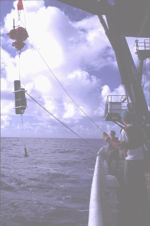
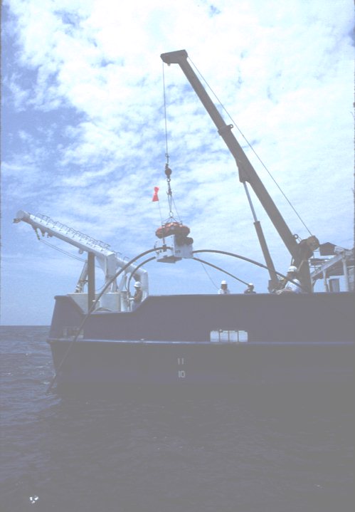
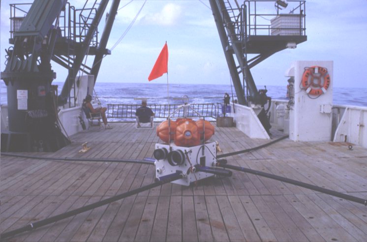
The new modular L-CHEAPO, shown here in the magnetotelluric configuration. This instrument has been tested in deep water on the April SWELL cruise and has been successfully deployed in experiments in the Gulf of Mexico.

top

E: The Seismic Part

Earlier seismic surface wave studies have found that the Hawaiian Swell may not be underlain by slow-velocity lithosphere, suggesting that lithosphere reheating is not the mechanism that leads to swell relief. These studies are based on the two-station method, in which surface waves are analyzed that travelled along the great circle of an event and two stations. Such analyses may be biased by effects of waves travelling in laterally heterogenous structure.

age groups: 4- 20 myrs
           20- 52 myrs
           52-110 myrs
           >  110 myrs

(above, left hand side) Shear velocity models for oceanic lithosphere as a function of age (Nishimura and Forsyth, 1989).
(right hand side) Group and phase velocities evaluated for the corresponding models on the left. Note that the line conventions in all 3 panels of this figure are the same.

Resolution kernels obtained using the Backus-Gilbert method for various target depths (vertical bars). The 'data' used for the resolution test are phase velocities from 15-60s. The resolution kernels for depths > 80km vary significantly when data between 40-60s are omitted (not shown here). This indicates that data between 40-60s are necessary to resolve (sub-lithospheric) structure below 80km. Due to the increased long-period noise induced by ocean gravity waves, useful signal above 60s will only be obtained for the largest earthquakes (Ms > 7.0).

top

F: The Magnetotelluric Part

Mantle electric conductivity is strongly influenced by temperature, hence conductivity structure at sub-lithospheric depths can easily be mapped using the magnetotelluric method. Apart from aiding and supporting the seismic experiment, the MT method has sensitivity similar to that of the seismic method, suggesting exciting possibilities for joint inversions.

Electrical model of generic plume and swell structure. Resistivity values are based on controlled source EM soundings, marine MT soundings, and laboratory studies of melt and subsolidus mantle rocks.

Magnetotelluric response of the swell model shown on the left. The wedge of reheated lithosphere/entrained plume is clearly visible in the data, particularly the E-W induced apparent resistivities. Omitting the wedge of relatively conductive material produces a much smaller response (at least factor two) localized around the narrow plume.

top

G: References

Von Herzen, R.P., et al., Heat flow and the thermal origin of hotspot swells: the Hawaiian Swell revisited, J. Geophys. Res. 94, 13,783-13,799, 1989.

Laske, G. and G. Masters, Constraints on global phase velocity maps from long-period polarization data, J. Geophys. Rres, 16,059-16,075,1996.

Ekstrom, G., J. Tromp and E. Larson, Measurements and global models of surface wave propagation, J. Geophys. Res., in press, 1997.

Trampert, J. and J.H. Woodhouse, High-resolution global phase velocity distributions, Geophys. Res. Let., 23, 21-24, 1996.

Zhang, Y.-S. and T. Lay, Global surface wave phase velocity variations, J. Geophys. Res., 101, 8415-8436, 1996.

Nishimura, C.E. and D.W. Forsyth, The anisotropic structure of the upper mantle in the Pacific, Geophys. J. Int. 96, 203-229, 1989.

top

This project has been presented at the following meetings:

IASPEI 29th General Assembly, August 18-28, 1997, Thessaloniki, Greece

AGU Spring 98 meeting, May 26-29, 1998, Boston

AGU Fall 98 meeting, December 6-10, 1998, San Francisco

IUGG 22nd General Assembly, July 18-30, 1999, Birmingham, England

AGU Fall 99 meeting, Dec 13-17, 1999, San Francisco

SSA 95th Annual Meeting, Apr 10-12, 2000, San Diego

12th Annual IRIS Workshop, May 09-11, 2000, Samoset Resort, Maine

PLUME 3 Conference, Jun 18-24, 2000, Four Seasons Resort, Hawaii

AGU Fall 2000 meeting, Dec 15-19, 2000, San Francisco

This research is funded by the National Science Foundation.

Gabi Laske ( glaske@ucsd.edu)

Goto U.S. OBS Instrument Pool (OBSIP) home page

Goto Gabi's Home page

To IGPP Home